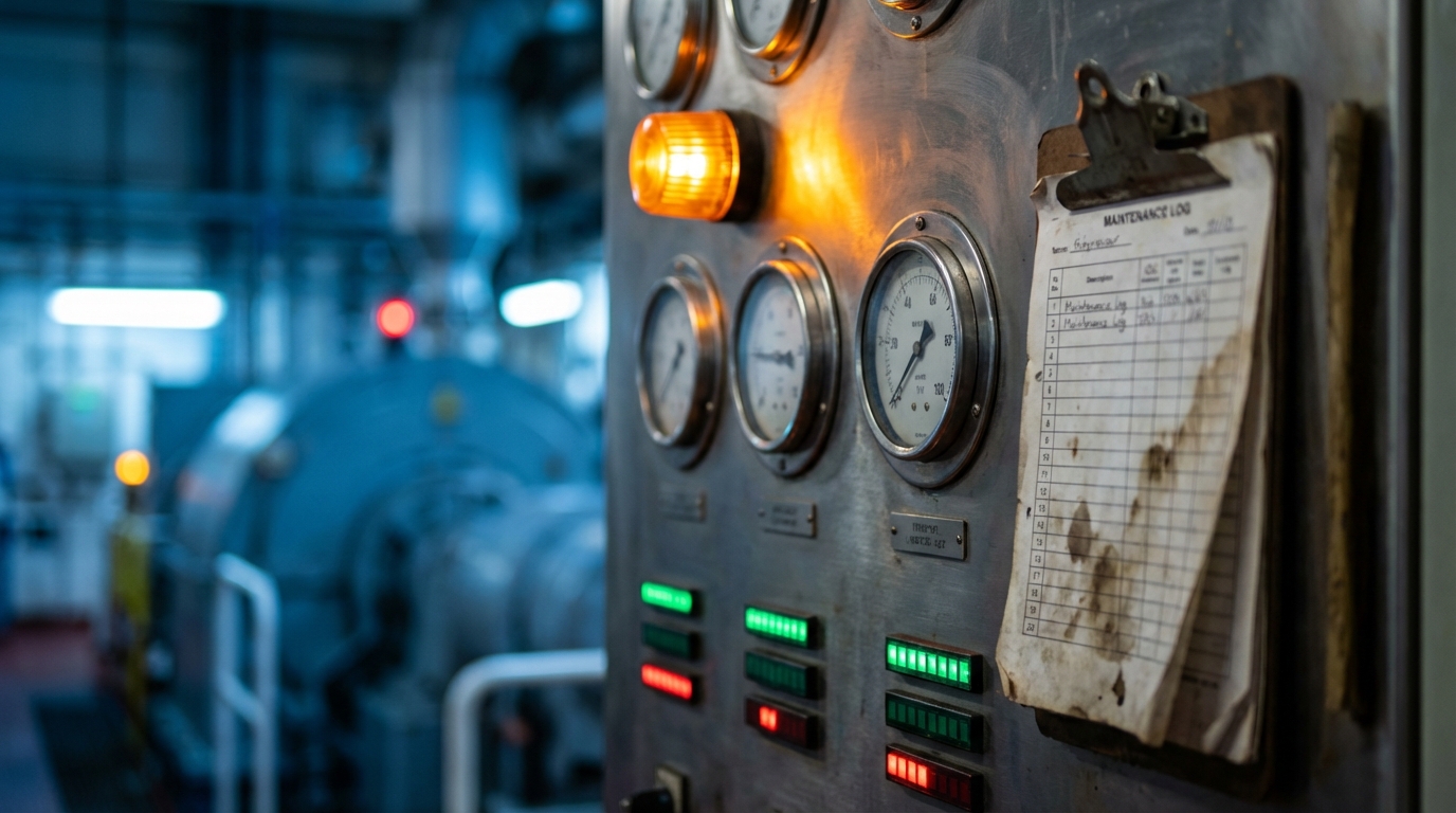
The Problem with "Run to Failure"
A compressor fails offshore at 2 a.m. The production train shuts down. By the time a crew mobilises, inspects, and sources the parts, you've lost three days of production. At $500K/day on a mid-size platform, that's $1.5M — for a failure that was visible in the sensor data a week before it happened.
Most operations teams still rely on one of two maintenance strategies:
- Time-based: Replace parts every N hours regardless of condition. Safe, but wasteful — you're discarding 30–40% of remaining useful life on average.
- Run to failure: Cheaper upfront, catastrophically expensive when it goes wrong.
Condition-based maintenance is the third path: predict when equipment will fail, service it at the right time, not the scheduled time. This article shows you how to build the prediction engine.
What is Remaining Useful Life?
Remaining Useful Life (RUL) is a single number: how many operational cycles does this piece of equipment have left before it needs maintenance?
Instead of asking "is this compressor OK right now?", RUL asks "how much life does it have left?" That shifts your maintenance team from reactive to proactive.
A RUL model takes a window of recent sensor readings as input and outputs a number — cycles remaining. Green means healthy, yellow means schedule maintenance, red means act now.
Why NASA's Turbofan Data Translates to Oil & Gas
The standard benchmark for RUL research is NASA's CMAPSS dataset (Commercial Modular Aero-Propulsion System Simulation). It simulates turbofan engine degradation with 21 sensors across hundreds of run-to-failure cycles.
Here's what's worth knowing: CMAPSS is itself synthetic. It's a validated physics simulation, not flight recorder data. This actually makes it ideal for methodology validation — the degradation patterns are clean, the physics are well-understood, and it's freely available.
More importantly, the degradation signatures — gradual drift in temperature, pressure, and flow sensors as components wear — are the same patterns seen in:
| CMAPSS sensor | O&G equivalent |
|---|---|
| Inlet temperature (s2) | Compressor suction temperature |
| Discharge temperature (s3) | Compressor discharge temperature |
| Discharge pressure (s7) | Discharge pressure (kPa) |
| Shaft speed (s8) | RPM |
| Flow ratio (s12) | Production flow ratio |
| Bypass ratio (s15) | Recycle ratio |
The physics differ in scale and medium. The signal processing is identical.
The Model: LSTM in 20 Lines
Long Short-Term Memory (LSTM) networks are designed for exactly this kind of problem: sequential data where the trend over time matters more than any single reading.
A compressor sensor reading at cycle 150 means nothing in isolation. That same reading after watching the temperature climb 8% over the past 30 cycles tells you everything.
import torch.nn as nn

class RUL_LSTM(nn.Module):
    def __init__(self, input_size=14, hidden_size=64, num_layers=2, dropout=0.2):
        super().__init__()
        self.lstm = nn.LSTM(
            input_size, hidden_size, num_layers,
            batch_first=True, dropout=dropout
        )
        self.dropout = nn.Dropout(dropout)
        self.fc = nn.Linear(hidden_size, 1)

    def forward(self, x):
        # x shape: (batch, 30 cycles, 14 sensors)
        _, (h_n, _) = self.lstm(x)
        return self.fc(self.dropout(h_n[-1]))
That's it. Input: a 30-cycle window of 14 sensor channels. Output: one number — predicted RUL.
Architecture details:
- 2 LSTM layers with 64 hidden units each
- Dropout 0.2 for regularisation
- MSE loss — standard for regression
- Trained with Adam, lr=1e-3, 60 epochs
Typical performance on the NASA FD001 test set: RMSE ~17–20 cycles, MAE ~12–14 cycles.
Preprocessing: Three Things That Actually Matter
1. Feature selection
CMAPSS has 21 sensors, but 7 of them are nearly constant across all operating conditions — no information, just noise. We use the 14 informative sensors identified in the literature:
SENSOR_COLS = ["s2", "s3", "s4", "s7", "s8", "s9", "s11",
               "s12", "s13", "s14", "s15", "s17", "s20", "s21"]
2. RUL clipping
At the start of an engine's life, the RUL might be 300 cycles — but the sensor data looks essentially the same at 300 cycles as at 150 cycles. The model can't learn anything useful from predicting "very healthy" vs "also very healthy."
Standard practice: clip RUL at 130 cycles. The model only needs to distinguish the last ~130 cycles before failure. Everything before that is labelled 130 (maximum health).
df["RUL"] = df["RUL"].clip(upper=130)
3. Normalisation
MinMaxScaler fitted on training data only, applied to both train and test. Don't leak test statistics into training.
Sliding Windows
Each training sample is a 30-cycle window of sensor readings with the RUL at the final cycle as the label:
cycles 1–30  → label: RUL at cycle 30
cycles 2–31  → label: RUL at cycle 31
...
cycles N-29–N → label: RUL at cycle N (= 0, failure)
This gives thousands of training samples from even a small number of run-to-failure engines.
The Live Demo
The demo is deployed at https://royabes-equipment-rul.streamlit.app/
It runs entirely on synthetic degradation data — no real NASA files required. Ten virtual equipment units are sampled at various lifecycle stages, from freshly commissioned (RUL ~100+) to near end-of-life (RUL <20).
Fleet Overview: A horizontal bar chart shows all units colour-coded by health:
- Green (RUL > 80): Healthy — normal operation
- Yellow (RUL 40–80): Monitor — schedule inspection
- Red (RUL < 40): Critical — act now
Unit Drill-down: Select any unit to see its sensor trend over the last 30 cycles and a RUL gauge showing life remaining as a percentage.
Upload Your Data: The "Upload Your Data" tab accepts a CSV with your own sensor readings and runs predictions against the pre-trained model. A template CSV is available for download.
Upload Your Own Sensor Data
The upload interface expects 16 columns:
unit_id, cycle, temp_inlet, temp_outlet, temp_exhaust,
pressure_discharge, speed_shaft, speed_core, pressure_static,
flow_rate, speed_corrected, speed_secondary, bypass_ratio,
bleed_enthalpy, coolant_1, coolant_2
Each row is one cycle of sensor readings for one piece of equipment. Multiple units can be in the same file — just use different unit_id values.
The model needs at least 30 cycles of history per unit. If you have fewer, the early cycles are padded.
From Demo to Production
The demo is a proof of concept. Here's what a production deployment looks like:
Data pipeline: OSIsoft PI / OPC-UA historian → feature extraction → 30-cycle sliding buffer per asset
Model serving: FastAPI endpoint wrapping the LSTM inference. The /predict route accepts a JSON payload of sensor readings and returns {unit_id, predicted_rul, status}.
Retraining: The model should be retrained as run-to-failure events accumulate on your actual equipment. Even 5–10 real failure cases will significantly outperform pure simulation data.
Uncertainty: Production deployments benefit from ensemble methods (multiple models with different seeds) or Bayesian approaches to quantify prediction uncertainty. A point estimate of "RUL = 45 cycles" is less useful than "RUL = 45 ± 12 cycles (95% CI)."
Honest Limitations
- Domain shift is real. A model trained on turbofan simulation will need recalibration on compressor data. The architecture transfers; the weights don't.
- Failure modes vary. CMAPSS FD001 has a single failure mode. Real equipment fails in many ways. A production system needs failure-mode classification alongside RUL prediction.
- Data quality matters. Missing sensors, sensor drift, and instrument faults degrade prediction quality faster than model complexity helps it.
Key Takeaways
- RUL prediction is achievable with public data. CMAPSS gives you a validated starting point without needing proprietary failure data.
- LSTMs handle temporal sensor data well. The 30-cycle window approach is simple and effective.
- Three preprocessing decisions dominate model quality: feature selection, RUL clipping, and proper normalisation.
- Sensor physics generalise. Degradation signatures in turbofan simulations map directly to compressors, pumps, and motors.
- The gap from demo to production is architecture, not algorithms. The ML is the easy part; data pipelines and reliability engineering are the hard part.
Resources
- Live demo: https://royabes-equipment-rul.streamlit.app/
- Source code: https://github.com/royabes/equipment-rul
- NASA CMAPSS dataset: https://data.nasa.gov/dataset/cmapss-jet-engine-simulated-data
The model weights and scaler in the repository are pre-trained on synthetic CMAPSS-style data. Clone the repo, run python train.py with the real NASA files, and you'll have a model ready to evaluate against your own equipment data.